Blog Post 3 - Fake News Classification

In this blog post, I’ll create a machine learning model for classifying fake news using Tensorflow supported by python. By using the python dataset, we’ll use the general format of kaggle dataset created by python.

Note: for the tutorial of Tensorflow, refer’s to PIC16B Tensorflow Course Notes by Phil.

Preparation: Import Packages

Before all, want to first import necessary python packages for the model creation

import numpy as np
import pandas as pd
import tensorflow as tf
import re
import string

from tensorflow.keras import layers
from tensorflow.keras import losses

# requires update to tensorflow 2.4
# >>> conda activate PIC16B
# >>> pip install tensorflow==2.4
from tensorflow.keras.layers.experimental.preprocessing import TextVectorization
from tensorflow.keras.layers.experimental.preprocessing import StringLookup

from sklearn.model_selection import train_test_split
from sklearn.preprocessing import LabelEncoder

# for embedding viz
import plotly.express as px 
import plotly.io as pio
pio.templates.default = "plotly_white"

# Part II imports
import tensorflow as tf
import nltk
nltk.download('stopwords')
from nltk.corpus import stopwords

# Part III imports
from tensorflow import keras
from matplotlib import pyplot as plt

# Part V imports
from sklearn.decomposition import PCA
import plotly.express as px

from plotly.io import write_html

Part I: Acquire Training Data

First, acquire the training data from the url provided below stored inside the variable train_url.

train_url = "https://github.com/PhilChodrow/PIC16b/blob/master/datasets/fake_news_train.csv?raw=true"
df  = pd.read_csv(train_url)

Now, visualize the dataset. The dataset should have three main contents with lots of observations. Each observation represents a piece of news. The three useful contents of the dataset are:

title: the title of the news piece
text: the main content / text of the news piece
fake: tell whether the news is fake (0: not fake, 1: fake)

The dataset is visualized as follows:

df.head()

	Unnamed: 0	title	text	fake
0	17366	Merkel: Strong result for Austria's FPO 'big c...	German Chancellor Angela Merkel said on Monday...	0
1	5634	Trump says Pence will lead voter fraud panel	WEST PALM BEACH, Fla.President Donald Trump sa...
2	17487	JUST IN: SUSPECTED LEAKER and “Close Confidant...	On December 5, 2017, Circa s Sara Carter warne...	1
3	12217	Thyssenkrupp has offered help to Argentina ove...	Germany s Thyssenkrupp, has offered assistance...	0
4	5535	Trump say appeals court decision on travel ban...	President Donald Trump on Thursday called the ...	0

Part II: Data Preparation

2.1 Prepare and Create Tensorflow Dataset

In this part, two tasks are operated:

Remove stopwords from title and text columns in the dataset
Convert the dataset to a Tensorflow-ready dataset

def make_dataset(df):
  """
  clean and remove stopwords from title and text and
  output it as a tensorflow dataset, the dataset has
  input contents as title and text, and output
  content as fake.

  Input
  --------
  df: the fake news dataset

  Output
  --------
  data: the described tensorflow dataset
  """

  # Step 1: Remove Stopwords from text and title
  test = df[['title', 'text', 'fake']] # get the useful parts of the input dataset
  stop = stopwords.words('english') # only want those english stopwords

  # remove stopwords on each targeting columns
  test["title"].str.split().apply(lambda x: " ".join([item for item in x if item not in stop]))
  test["text"].str.split().apply(lambda x: " ".join([item for item in x if item not in stop]))

  # Step 2: prepare the tensorflow dataset
  data = tf.data.Dataset.from_tensor_slices(
    (
        {
            "title" : test[["title"]], 
            "text" : test[["text"]]
        }, 
        {
            "fake" : test[["fake"]]
        }
    )
  )
  # return, choose a nice batching
  return data.batch(100)

In the peer feedback, two of my peers mentioned that the original for-loop in this function can actually be removed. Therefore, I went back to see whether my function was having the issue. From the observation, I think the for-loop is actually fine as it just represents the title and text column for looping. However, I observed that in the loops, I got an redundant step to bring the strings together. One of my peers said that the redundant step is possible to remove by directly doing string split. Therefore, I tried to add the commands directly after doing str.split(). Below is the original version I’ve wrote for this function.

def make_dataset(df):
  """
  clean and remove stopwords from title and text and
  output it as a tensorflow dataset, the dataset has
  input contents as title and text, and output
  content as fake.

  Input
  --------
  df: the fake news dataset

  Output
  --------
  data: the described tensorflow dataset
  """

  # Step 1: Remove Stopwords from text and title
  test = df[['title', 'text', 'fake']] # get the useful parts of the input dataset
  test.col = ['title', 'text'] # columns for removing stopwords
  stop = stopwords.words('english') # only want those english stopwords

  # remove stopwords on each targeting columns
  for col in test.col:
    # split string
    test[col] = test[col].str.split()
    # move stopwords
    test[col].apply(lambda x: " ".join([item for item in x if item not in stop]))
    # rejoin strings
    test[col] = [" ".join(string) for string in test[col]]

  # Step 2: prepare the tensorflow dataset
  data = tf.data.Dataset.from_tensor_slices(
    (
        {
            "title" : test[["title"]], 
            "text" : test[["text"]]
        }, 
        {
            "fake" : test[["fake"]]
        }
    )
  )
  # return, choose a nice batching
  return data.batch(100)

Also, one of my peers mentioned that I did not do the lowercase remove. Although my peer mentioned this one as a potential error, I am actually removing this lowercase command in purpose, as the score is higher for the version without converting to lowercase. For possible reasoning, please see the content in part VI.

2.2 Train-Validation Separation

Now, first use the function in 2.1 to construct a tensorflow-valid dataset, store it as data:

data = make_dataset(df)

Next, split of 20% of it to use for validation. Here, first create a function train_test_split() to do train-validation splitting.

def train_test_split(data):
  """
  split a tensorflow dataset into 80:20 train:validation,
  and output train and validation

  Input
  --------
  dataset: the whole tensorflow dataset
  Output
  --------
  (train, val): training and validation datasets
  """
  np.random.seed(9999)

  data = data.shuffle(buffer_size = len(data))

  val_size = int(0.2*len(data)) # the split is 80-20 training-validation

  val = data.take(val_size)
  train   = data.skip(val_size)

  return (train, val)

Now, do the 20% validation splitting, store the two contents as train and validation.

train, validation = train_test_split(data)

For confirming, see number of observations in each set:

len(train), len(validation)

(180, 45)

From the result, confirmed.

Part III: Model Creation and Comparison

In this section, want to confirm whether the Tensorflow fake news classifier model is better working on only title data, only text data, or both

To satisfy the goal, I’ll create three separate Tensorflow model in this part, with different input streams: model 1 only with title data, model 2 only with text data, and model 3 with both

3.0 Model Preparation

Before create and analyze three models, there are some preparation work to do.

First, do the standardization and vectorization on the train dataset.

This is the function for doing standardization on a input dataset

Note this standardization function is created as an input parameter for the hyperparameter standardize in the TextVectorization, which is used below.

def standardization(input_data):
    lowercase = tf.strings.lower(input_data)
    no_punctuation = tf.strings.regex_replace(lowercase,
                                  '[%s]' % re.escape(string.punctuation),'')
    return no_punctuation

Now, do the text vectorization

Note that for using the python-supported function TextVectorization(), want to specify two specific hyperparameters max_tokens and output_sequence_length. Here, use:

max_tokens = 2000: only the top 2000 words will be tracked
output_sequence_length = 500: each headline will be a vector of length 500

size_vocabulary = 2000 # max_tokens specifier

vectorize_layer = TextVectorization(
  standardize=standardization,
  max_tokens=size_vocabulary, # only consider this many words
  output_mode='int',
  output_sequence_length=500) 

vectorize_layer.adapt(train.map(lambda x, y: x["title"] + x["text"]))

Now, specify the input parameter for title and text, store them as titles_input and texts_input.

titles_input = keras.Input(
    shape = (1,), 
    name = "title",
    dtype = "string"
)

texts_input = keras.Input(
    shape = (1,), 
    name = "text",
    dtype = "string"
)

3.1 Model 1: Title-Only Analysis

This model is created with text information only in the titles of fake news.

First, create the layers and output parameter of the model, store the output parameter as titles_output. The input is previously specified titles_input parameter.

# layers for processing the title, pretty much the same as from our lecture
# on text classification
titles_features = vectorize_layer(titles_input)
titles_features = layers.Embedding(size_vocabulary, 3, name = "title_only")(titles_features)
titles_features = layers.Dropout(0.2)(titles_features)
titles_features = layers.GlobalAveragePooling1D()(titles_features)
titles_features = layers.Dropout(0.2)(titles_features)
titles_features = layers.Dense(32, activation='relu')(titles_features)
# create output
titles_output = layers.Dense(2, name = "fake")(titles_features)

Now, create the model:

titles_model = keras.Model(
    inputs = titles_input,
    outputs = titles_output
)

Here is the model summary:

# model result
titles_model.summary()

Model: "model_1"
_________________________________________________________________
Layer (type)                 Output Shape              Param #   
=================================================================
title (InputLayer)           [(None, 1)]               0         
_________________________________________________________________
text_vectorization_1 (TextVe (None, 500)               0         
_________________________________________________________________
title_only_embedding (Embedd (None, 500, 3)            6000      
_________________________________________________________________
dropout_4 (Dropout)          (None, 500, 3)            0         
_________________________________________________________________
global_average_pooling1d_2 ( (None, 3)                 0         
_________________________________________________________________
dropout_5 (Dropout)          (None, 3)                 0         
_________________________________________________________________
dense_2 (Dense)              (None, 32)                128       
_________________________________________________________________
fake (Dense)                 (None, 2)                 66        
=================================================================
Total params: 6,194
Trainable params: 6,194
Non-trainable params: 0
_________________________________________________________________

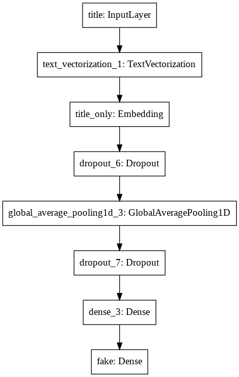
And here is the model flow diagram:

# model flow
keras.utils.plot_model(titles_model)

Now, compile and train the model with results showing after every epoch:

# compile
titles_model.compile(optimizer = "adam",
              loss = losses.SparseCategoricalCrossentropy(from_logits=True),
              metrics=['accuracy']
)

# train
titles_history = titles_model.fit(train, 
                    validation_data=validation,
                    epochs = 30)

Epoch 1/30
/usr/local/lib/python3.7/dist-packages/tensorflow/python/keras/engine/functional.py:595: UserWarning:

Input dict contained keys ['text'] which did not match any model input. They will be ignored by the model.

180/180 [==============================] - 2s 10ms/step - loss: 0.6926 - accuracy: 0.5179 - val_loss: 0.6910 - val_accuracy: 0.5271
Epoch 2/30
180/180 [==============================] - 2s 9ms/step - loss: 0.6885 - accuracy: 0.5305 - val_loss: 0.6737 - val_accuracy: 0.5193
Epoch 3/30
180/180 [==============================] - 2s 9ms/step - loss: 0.6574 - accuracy: 0.6606 - val_loss: 0.5898 - val_accuracy: 0.8503
Epoch 4/30
180/180 [==============================] - 2s 9ms/step - loss: 0.5590 - accuracy: 0.8332 - val_loss: 0.4553 - val_accuracy: 0.8847
Epoch 5/30
180/180 [==============================] - 2s 8ms/step - loss: 0.4346 - accuracy: 0.8744 - val_loss: 0.3441 - val_accuracy: 0.8967
Epoch 6/30
180/180 [==============================] - 2s 8ms/step - loss: 0.3473 - accuracy: 0.8878 - val_loss: 0.2788 - val_accuracy: 0.9164
Epoch 7/30
180/180 [==============================] - 2s 9ms/step - loss: 0.2957 - accuracy: 0.8895 - val_loss: 0.2414 - val_accuracy: 0.9231
Epoch 8/30
180/180 [==============================] - 2s 8ms/step - loss: 0.2636 - accuracy: 0.9031 - val_loss: 0.2076 - val_accuracy: 0.9324
Epoch 9/30
180/180 [==============================] - 2s 9ms/step - loss: 0.2444 - accuracy: 0.9099 - val_loss: 0.1951 - val_accuracy: 0.9313
Epoch 10/30
180/180 [==============================] - 2s 8ms/step - loss: 0.2188 - accuracy: 0.9184 - val_loss: 0.1793 - val_accuracy: 0.9416
Epoch 11/30
180/180 [==============================] - 2s 9ms/step - loss: 0.2047 - accuracy: 0.9228 - val_loss: 0.1693 - val_accuracy: 0.9418
Epoch 12/30
180/180 [==============================] - 2s 9ms/step - loss: 0.1945 - accuracy: 0.9282 - val_loss: 0.1689 - val_accuracy: 0.9411
Epoch 13/30
180/180 [==============================] - 2s 8ms/step - loss: 0.1978 - accuracy: 0.9240 - val_loss: 0.1714 - val_accuracy: 0.9364
Epoch 14/30
180/180 [==============================] - 2s 8ms/step - loss: 0.1901 - accuracy: 0.9290 - val_loss: 0.1468 - val_accuracy: 0.9449
Epoch 15/30
180/180 [==============================] - 2s 8ms/step - loss: 0.1785 - accuracy: 0.9329 - val_loss: 0.1395 - val_accuracy: 0.9464
Epoch 16/30
180/180 [==============================] - 2s 9ms/step - loss: 0.1748 - accuracy: 0.9347 - val_loss: 0.1389 - val_accuracy: 0.9480
Epoch 17/30
180/180 [==============================] - 2s 8ms/step - loss: 0.1775 - accuracy: 0.9339 - val_loss: 0.1381 - val_accuracy: 0.9496
Epoch 18/30
180/180 [==============================] - 2s 8ms/step - loss: 0.1632 - accuracy: 0.9401 - val_loss: 0.1449 - val_accuracy: 0.9440
Epoch 19/30
180/180 [==============================] - 1s 8ms/step - loss: 0.1718 - accuracy: 0.9314 - val_loss: 0.1335 - val_accuracy: 0.9512
Epoch 20/30
180/180 [==============================] - 2s 8ms/step - loss: 0.1645 - accuracy: 0.9392 - val_loss: 0.1268 - val_accuracy: 0.9520
Epoch 21/30
180/180 [==============================] - 2s 8ms/step - loss: 0.1602 - accuracy: 0.9371 - val_loss: 0.1357 - val_accuracy: 0.9487
Epoch 22/30
180/180 [==============================] - 1s 8ms/step - loss: 0.1471 - accuracy: 0.9455 - val_loss: 0.1174 - val_accuracy: 0.9587
Epoch 23/30
180/180 [==============================] - 2s 8ms/step - loss: 0.1557 - accuracy: 0.9419 - val_loss: 0.1336 - val_accuracy: 0.9464
Epoch 24/30
180/180 [==============================] - 2s 8ms/step - loss: 0.1592 - accuracy: 0.9404 - val_loss: 0.1178 - val_accuracy: 0.9564
Epoch 25/30
180/180 [==============================] - 2s 8ms/step - loss: 0.1484 - accuracy: 0.9433 - val_loss: 0.1205 - val_accuracy: 0.9551
Epoch 26/30
180/180 [==============================] - 1s 8ms/step - loss: 0.1460 - accuracy: 0.9441 - val_loss: 0.1221 - val_accuracy: 0.9556
Epoch 27/30
180/180 [==============================] - 2s 8ms/step - loss: 0.1499 - accuracy: 0.9417 - val_loss: 0.1207 - val_accuracy: 0.9544
Epoch 28/30
180/180 [==============================] - 2s 8ms/step - loss: 0.1468 - accuracy: 0.9430 - val_loss: 0.1193 - val_accuracy: 0.9564
Epoch 29/30
180/180 [==============================] - 2s 8ms/step - loss: 0.1462 - accuracy: 0.9440 - val_loss: 0.1123 - val_accuracy: 0.9591
Epoch 30/30
180/180 [==============================] - 2s 8ms/step - loss: 0.1435 - accuracy: 0.9445 - val_loss: 0.1148 - val_accuracy: 0.9580

From the result, can see that after epoch #19, the validation accuracy stablized around 95%, indicating a constantly okay validation score. Therefore, the model could correctly predict 95% of news correctly on whether the given news is fake.

To see the training and validation score history with epoch, plot the score history plot:

plt.plot(titles_history.history["accuracy"], label = "training accuracy")
plt.plot(titles_history.history["val_accuracy"], label = "validation accuracy")
plt.plot([0,30], [0.95,0.95], "r--", label = "95% accuracy")
plt.xlabel('Number of Epoch')
plt.ylabel('Accuracy')
plt.title('Training Result of Title-Only Model')
plt.legend()

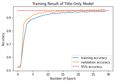
My suggestion: maybe add a 95% accuracy horizontal line to see the training and validation accuracy bondary, as this might be easier for readers to see, as some of the graph are not printing specified boundaries above 0.9 accuracy.

3.2 Model 2: Text-Only Analysis

This model is created with text information only in the text sections of fake news.

First, create the layers and output parameter of the model, store the output parameter as texts_output. The input is previously specified texts_input parameter.

# layers for processing the text, pretty much the same as from our lecture
# on text classification
texts_features = vectorize_layer(texts_input)
texts_features = layers.Embedding(size_vocabulary, 3, name = "text_only")(texts_features)
texts_features = layers.Dropout(0.2)(texts_features)
texts_features = layers.GlobalAveragePooling1D()(texts_features)
texts_features = layers.Dropout(0.2)(texts_features)
texts_features = layers.Dense(32, activation='relu')(texts_features)
# create output
texts_output = layers.Dense(2, name = "fake")(texts_features)

Now, create the model:

texts_model = keras.Model(
    inputs = texts_input,
    outputs = texts_output
)

Here is the model summary:

# model result
texts_model.summary()

Model: "model_2"
_________________________________________________________________
Layer (type)                 Output Shape              Param #   
=================================================================
text (InputLayer)            [(None, 1)]               0         
_________________________________________________________________
text_vectorization_1 (TextVe (None, 500)               0         
_________________________________________________________________
text_only (Embedding)        (None, 500, 3)            6000      
_________________________________________________________________
dropout_8 (Dropout)          (None, 500, 3)            0         
_________________________________________________________________
global_average_pooling1d_4 ( (None, 3)                 0         
_________________________________________________________________
dropout_9 (Dropout)          (None, 3)                 0         
_________________________________________________________________
dense_4 (Dense)              (None, 32)                128       
_________________________________________________________________
fake (Dense)                 (None, 2)                 66        
=================================================================
Total params: 6,194
Trainable params: 6,194
Non-trainable params: 0
_________________________________________________________________

And here is the model flow diagram:

# model flow
keras.utils.plot_model(texts_model)

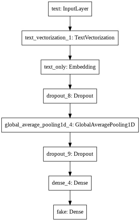
In the peers feedback, one of my peer mentioned that I did not change the name of embedding layer to specify the difference between model_1 and model_2, before changing, my code for model_1 and model_2 are:

# model 1
titles_features = layers.Embedding(size_vocabulary, 3, name = "embedding")(titles_features)
# model 2
texts_features = layers.Embedding(size_vocabulary, 3, name = "embedding")(texts_features)

Therefore, I changed the two lines into:

# model 1
titles_features = layers.Embedding(size_vocabulary, 3, name = "title_only")(titles_features)
# model 2
texts_features = layers.Embedding(size_vocabulary, 3, name = "text_only")(texts_features)

and then change the corresponding model summary and flows diagram.

Now, compile and train the model with results showing after every epoch:

# compile
texts_model.compile(optimizer = "adam",
              loss = losses.SparseCategoricalCrossentropy(from_logits=True),
              metrics=['accuracy']
)

# train
texts_history = texts_model.fit(train, 
                    validation_data=validation,
                    epochs = 30)

Epoch 1/30
/usr/local/lib/python3.7/dist-packages/tensorflow/python/keras/engine/functional.py:595: UserWarning:

Input dict contained keys ['title'] which did not match any model input. They will be ignored by the model.

180/180 [==============================] - 4s 21ms/step - loss: 0.6853 - accuracy: 0.5435 - val_loss: 0.5913 - val_accuracy: 0.8413
Epoch 2/30
180/180 [==============================] - 4s 19ms/step - loss: 0.5224 - accuracy: 0.8622 - val_loss: 0.3184 - val_accuracy: 0.9473
Epoch 3/30
180/180 [==============================] - 4s 19ms/step - loss: 0.2948 - accuracy: 0.9278 - val_loss: 0.1962 - val_accuracy: 0.9573
Epoch 4/30
180/180 [==============================] - 4s 19ms/step - loss: 0.2009 - accuracy: 0.9490 - val_loss: 0.1485 - val_accuracy: 0.9680
Epoch 5/30
180/180 [==============================] - 4s 20ms/step - loss: 0.1582 - accuracy: 0.9597 - val_loss: 0.1225 - val_accuracy: 0.9707
Epoch 6/30
180/180 [==============================] - 4s 19ms/step - loss: 0.1350 - accuracy: 0.9656 - val_loss: 0.1091 - val_accuracy: 0.9736
Epoch 7/30
180/180 [==============================] - 3s 19ms/step - loss: 0.1203 - accuracy: 0.9684 - val_loss: 0.0956 - val_accuracy: 0.9782
Epoch 8/30
180/180 [==============================] - 3s 19ms/step - loss: 0.1052 - accuracy: 0.9722 - val_loss: 0.0882 - val_accuracy: 0.9776
Epoch 9/30
180/180 [==============================] - 3s 19ms/step - loss: 0.0964 - accuracy: 0.9757 - val_loss: 0.0854 - val_accuracy: 0.9796
Epoch 10/30
180/180 [==============================] - 3s 19ms/step - loss: 0.0845 - accuracy: 0.9793 - val_loss: 0.0672 - val_accuracy: 0.9856
Epoch 11/30
180/180 [==============================] - 4s 20ms/step - loss: 0.0849 - accuracy: 0.9770 - val_loss: 0.0629 - val_accuracy: 0.9849
Epoch 12/30
180/180 [==============================] - 3s 19ms/step - loss: 0.0753 - accuracy: 0.9785 - val_loss: 0.0558 - val_accuracy: 0.9878
Epoch 13/30
180/180 [==============================] - 4s 19ms/step - loss: 0.0693 - accuracy: 0.9814 - val_loss: 0.0499 - val_accuracy: 0.9907
Epoch 14/30
180/180 [==============================] - 4s 19ms/step - loss: 0.0656 - accuracy: 0.9829 - val_loss: 0.0549 - val_accuracy: 0.9852
Epoch 15/30
180/180 [==============================] - 4s 20ms/step - loss: 0.0659 - accuracy: 0.9804 - val_loss: 0.0502 - val_accuracy: 0.9896
Epoch 16/30
180/180 [==============================] - 4s 20ms/step - loss: 0.0647 - accuracy: 0.9797 - val_loss: 0.0500 - val_accuracy: 0.9904
Epoch 17/30
180/180 [==============================] - 4s 20ms/step - loss: 0.0602 - accuracy: 0.9819 - val_loss: 0.0445 - val_accuracy: 0.9891
Epoch 18/30
180/180 [==============================] - 4s 20ms/step - loss: 0.0552 - accuracy: 0.9829 - val_loss: 0.0397 - val_accuracy: 0.9903
Epoch 19/30
180/180 [==============================] - 4s 20ms/step - loss: 0.0511 - accuracy: 0.9868 - val_loss: 0.0366 - val_accuracy: 0.9924
Epoch 20/30
180/180 [==============================] - 4s 20ms/step - loss: 0.0563 - accuracy: 0.9825 - val_loss: 0.0342 - val_accuracy: 0.9918
Epoch 21/30
180/180 [==============================] - 4s 20ms/step - loss: 0.0441 - accuracy: 0.9866 - val_loss: 0.0341 - val_accuracy: 0.9924
Epoch 22/30
180/180 [==============================] - 4s 20ms/step - loss: 0.0463 - accuracy: 0.9867 - val_loss: 0.0328 - val_accuracy: 0.9924
Epoch 23/30
180/180 [==============================] - 4s 20ms/step - loss: 0.0460 - accuracy: 0.9845 - val_loss: 0.0221 - val_accuracy: 0.9946
Epoch 24/30
180/180 [==============================] - 4s 19ms/step - loss: 0.0438 - accuracy: 0.9869 - val_loss: 0.0284 - val_accuracy: 0.9924
Epoch 25/30
180/180 [==============================] - 4s 20ms/step - loss: 0.0396 - accuracy: 0.9883 - val_loss: 0.0261 - val_accuracy: 0.9962
Epoch 26/30
180/180 [==============================] - 4s 19ms/step - loss: 0.0448 - accuracy: 0.9860 - val_loss: 0.0213 - val_accuracy: 0.9964
Epoch 27/30
180/180 [==============================] - 4s 20ms/step - loss: 0.0359 - accuracy: 0.9886 - val_loss: 0.0191 - val_accuracy: 0.9960
Epoch 28/30
180/180 [==============================] - 4s 20ms/step - loss: 0.0396 - accuracy: 0.9876 - val_loss: 0.0226 - val_accuracy: 0.9946
Epoch 29/30
180/180 [==============================] - 4s 20ms/step - loss: 0.0359 - accuracy: 0.9869 - val_loss: 0.0230 - val_accuracy: 0.9964
Epoch 30/30
180/180 [==============================] - 4s 20ms/step - loss: 0.0375 - accuracy: 0.9887 - val_loss: 0.0159 - val_accuracy: 0.9960

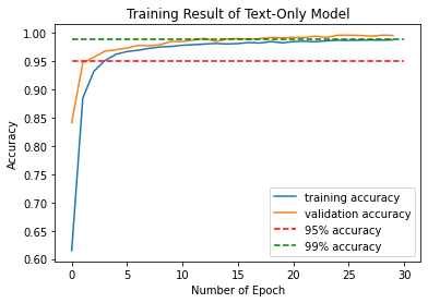
From the result, can see that after epoch #13, the validation accuracy stablized around 99%, indicating a constantly high validation score. Therefore, the model could correctly predict 99% of news correctly on whether the given news is fake.

To see the training and validation score history with epoch, plot the score history plot:

plt.plot(texts_history.history["accuracy"], label = "training accuracy")
plt.plot(texts_history.history["val_accuracy"], label = "validation accuracy")
plt.plot([0,30], [0.95,0.95], "r--", label = "95% accuracy")
plt.plot([0,30], [0.99,0.99], "g--", label = "99% accuracy")
plt.xlabel('Number of Epoch')
plt.ylabel('Accuracy')
plt.title('Training Result of Text-Only Model')
plt.legend()

3.3 Model 3: Title-Text Analysis

This model is created with text information only in the titles of fake news.

First, create the layers and output parameter of the model. For the combined model, need to first build the structure on titles and texts separately, and then concatenate them into a combined feature named main, and create output parameter from main.

Here, store the output parameter as output:

# 1. layers for processing the title, pretty much the same as from our lecture
titles_features = vectorize_layer(titles_input)
titles_features = layers.Embedding(size_vocabulary, 3, name = "titles")(titles_features)
titles_features = layers.Dropout(0.2)(titles_features)
titles_features = layers.GlobalAveragePooling1D()(titles_features)
titles_features = layers.Dropout(0.2)(titles_features)
titles_features = layers.Dense(32, activation='relu')(titles_features)

# 2. layers for processing the text, pretty much the same as from our lecture
texts_features = vectorize_layer(texts_input)
texts_features = layers.Embedding(size_vocabulary, 3, name = "texts")(texts_features)
texts_features = layers.Dropout(0.2)(texts_features)
texts_features = layers.GlobalAveragePooling1D()(texts_features)
texts_features = layers.Dropout(0.2)(texts_features)
texts_features = layers.Dense(32, activation='relu')(texts_features)

# 3. concatenate and create output
main = layers.concatenate([titles_features, texts_features], axis = 1)
main = layers.Dense(10, activation='relu')(main)
output = layers.Dense(2, name = "fake")(main)

Now, create the model:

combined_model = keras.Model(
    inputs = [titles_input, texts_input],
    outputs = output
)

Here is the model summary:

# model result
combined_model.summary()

Model: "model_4"
__________________________________________________________________________________________________
Layer (type)                    Output Shape         Param #     Connected to                     
==================================================================================================
title (InputLayer)              [(None, 1)]          0                                            
__________________________________________________________________________________________________
text (InputLayer)               [(None, 1)]          0                                            
__________________________________________________________________________________________________
text_vectorization_1 (TextVecto (None, 500)          0           title[0][0]                      
                                                                 text[0][0]                       
__________________________________________________________________________________________________
titles (Embedding)              (None, 500, 3)       6000        text_vectorization_1[3][0]       
__________________________________________________________________________________________________
texts (Embedding)               (None, 500, 3)       6000        text_vectorization_1[4][0]       
__________________________________________________________________________________________________
dropout_8 (Dropout)             (None, 500, 3)       0           titles[0][0]                     
__________________________________________________________________________________________________
dropout_10 (Dropout)            (None, 500, 3)       0           texts[0][0]                      
__________________________________________________________________________________________________
global_average_pooling1d_4 (Glo (None, 3)            0           dropout_8[0][0]                  
__________________________________________________________________________________________________
global_average_pooling1d_5 (Glo (None, 3)            0           dropout_10[0][0]                 
__________________________________________________________________________________________________
dropout_9 (Dropout)             (None, 3)            0           global_average_pooling1d_4[0][0] 
__________________________________________________________________________________________________
dropout_11 (Dropout)            (None, 3)            0           global_average_pooling1d_5[0][0] 
__________________________________________________________________________________________________
dense_4 (Dense)                 (None, 32)           128         dropout_9[0][0]                  
__________________________________________________________________________________________________
dense_5 (Dense)                 (None, 32)           128         dropout_11[0][0]                 
__________________________________________________________________________________________________
concatenate (Concatenate)       (None, 64)           0           dense_4[0][0]                    
                                                                 dense_5[0][0]                    
__________________________________________________________________________________________________
dense_6 (Dense)                 (None, 10)           650         concatenate[0][0]                
__________________________________________________________________________________________________
fake (Dense)                    (None, 2)            22          dense_6[0][0]                    
==================================================================================================
Total params: 12,928
Trainable params: 12,928
Non-trainable params: 0
__________________________________________________________________________________________________

And here is the model flow diagram:

# model flow
keras.utils.plot_model(combined_model)

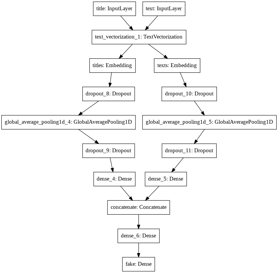
Now, compile and train the model with results showing after every epoch:

# compile
combined_model.compile(optimizer = "adam",
              loss = losses.SparseCategoricalCrossentropy(from_logits=True),
              metrics=['accuracy']
)

# train
combined_history = combined_model.fit(train, 
                    validation_data=validation,
                    epochs = 30)

Epoch 1/30
180/180 [==============================] - 6s 26ms/step - loss: 0.6908 - accuracy: 0.5340 - val_loss: 0.6094 - val_accuracy: 0.8527
Epoch 2/30
180/180 [==============================] - 4s 24ms/step - loss: 0.4641 - accuracy: 0.8840 - val_loss: 0.1796 - val_accuracy: 0.9542
Epoch 3/30
180/180 [==============================] - 4s 24ms/step - loss: 0.1742 - accuracy: 0.9483 - val_loss: 0.1185 - val_accuracy: 0.9696
Epoch 4/30
180/180 [==============================] - 4s 23ms/step - loss: 0.1277 - accuracy: 0.9634 - val_loss: 0.0914 - val_accuracy: 0.9760
Epoch 5/30
180/180 [==============================] - 4s 23ms/step - loss: 0.1029 - accuracy: 0.9733 - val_loss: 0.0719 - val_accuracy: 0.9820
Epoch 6/30
180/180 [==============================] - 4s 24ms/step - loss: 0.0861 - accuracy: 0.9759 - val_loss: 0.0601 - val_accuracy: 0.9833
Epoch 7/30
180/180 [==============================] - 4s 23ms/step - loss: 0.0663 - accuracy: 0.9821 - val_loss: 0.0451 - val_accuracy: 0.9896
Epoch 8/30
180/180 [==============================] - 4s 24ms/step - loss: 0.0568 - accuracy: 0.9838 - val_loss: 0.0443 - val_accuracy: 0.9887
Epoch 9/30
180/180 [==============================] - 4s 23ms/step - loss: 0.0490 - accuracy: 0.9866 - val_loss: 0.0299 - val_accuracy: 0.9924
Epoch 10/30
180/180 [==============================] - 4s 24ms/step - loss: 0.0458 - accuracy: 0.9879 - val_loss: 0.0342 - val_accuracy: 0.9906
Epoch 11/30
180/180 [==============================] - 4s 24ms/step - loss: 0.0384 - accuracy: 0.9903 - val_loss: 0.0328 - val_accuracy: 0.9902
Epoch 12/30
180/180 [==============================] - 4s 24ms/step - loss: 0.0324 - accuracy: 0.9905 - val_loss: 0.0301 - val_accuracy: 0.9903
Epoch 13/30
180/180 [==============================] - 4s 24ms/step - loss: 0.0355 - accuracy: 0.9903 - val_loss: 0.0203 - val_accuracy: 0.9951
Epoch 14/30
180/180 [==============================] - 4s 24ms/step - loss: 0.0303 - accuracy: 0.9918 - val_loss: 0.0159 - val_accuracy: 0.9964
Epoch 15/30
180/180 [==============================] - 4s 24ms/step - loss: 0.0274 - accuracy: 0.9926 - val_loss: 0.0138 - val_accuracy: 0.9958
Epoch 16/30
180/180 [==============================] - 4s 24ms/step - loss: 0.0223 - accuracy: 0.9942 - val_loss: 0.0116 - val_accuracy: 0.9976
Epoch 17/30
180/180 [==============================] - 4s 24ms/step - loss: 0.0195 - accuracy: 0.9941 - val_loss: 0.0116 - val_accuracy: 0.9971
Epoch 18/30
180/180 [==============================] - 4s 24ms/step - loss: 0.0193 - accuracy: 0.9942 - val_loss: 0.0092 - val_accuracy: 0.9982
Epoch 19/30
180/180 [==============================] - 4s 24ms/step - loss: 0.0163 - accuracy: 0.9951 - val_loss: 0.0088 - val_accuracy: 0.9982
Epoch 20/30
180/180 [==============================] - 4s 24ms/step - loss: 0.0173 - accuracy: 0.9946 - val_loss: 0.0086 - val_accuracy: 0.9976
Epoch 21/30
180/180 [==============================] - 4s 24ms/step - loss: 0.0189 - accuracy: 0.9949 - val_loss: 0.0064 - val_accuracy: 0.9982
Epoch 22/30
180/180 [==============================] - 4s 23ms/step - loss: 0.0153 - accuracy: 0.9948 - val_loss: 0.0055 - val_accuracy: 0.9991
Epoch 23/30
180/180 [==============================] - 4s 24ms/step - loss: 0.0167 - accuracy: 0.9941 - val_loss: 0.0085 - val_accuracy: 0.9962
Epoch 24/30
180/180 [==============================] - 4s 24ms/step - loss: 0.0156 - accuracy: 0.9961 - val_loss: 0.0042 - val_accuracy: 0.9998
Epoch 25/30
180/180 [==============================] - 4s 24ms/step - loss: 0.0133 - accuracy: 0.9955 - val_loss: 0.0064 - val_accuracy: 0.9989
Epoch 26/30
180/180 [==============================] - 4s 24ms/step - loss: 0.0116 - accuracy: 0.9965 - val_loss: 0.0100 - val_accuracy: 0.9973
Epoch 27/30
180/180 [==============================] - 4s 24ms/step - loss: 0.0130 - accuracy: 0.9957 - val_loss: 0.0057 - val_accuracy: 0.9993
Epoch 28/30
180/180 [==============================] - 4s 24ms/step - loss: 0.0124 - accuracy: 0.9954 - val_loss: 0.0087 - val_accuracy: 0.9982
Epoch 29/30
180/180 [==============================] - 4s 24ms/step - loss: 0.0116 - accuracy: 0.9966 - val_loss: 0.0048 - val_accuracy: 0.9989
Epoch 30/30
180/180 [==============================] - 4s 24ms/step - loss: 0.0102 - accuracy: 0.9964 - val_loss: 0.0043 - val_accuracy: 0.9993

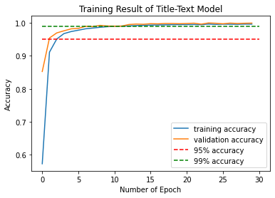
From the result, can see that after epoch #9, the validation accuracy stablized around 99%, indicating a constantly high validation score. Therefore, the model could correctly predict 99% of news correctly on whether the given news is fake.

To see the training and validation score history with epoch, plot the score history plot:

plt.plot(combined_history.history["accuracy"], label = "training accuracy")
plt.plot(combined_history.history["val_accuracy"], label = "validation accuracy")
plt.plot([0,30], [0.95,0.95], "r--", label = "95% accuracy")
plt.plot([0,30], [0.99,0.99], "g--", label = "99% accuracy")
plt.xlabel('Number of Epoch')
plt.ylabel('Accuracy')
plt.title('Training Result of Title-Text Model')
plt.legend()

3.4 Comparison and Selection

From the above results, could see that both model 2 and model 3 results in a constantly high validation score after several epochs of training. However, the validation accuracy of model 3 is constantly around 99.8% - 99.9% after 20 epoches, which is still higher than model 2. Therefore, could conclude that using both title and text content for news to train the Tensorflow fake news model results in highest level accuracy of recognizing fake news.

Part IV: Model Evaluation

In part III, I’ve concluded that model 3 with both text and title analysis results in the best prediction on fake news classification. In this part, I’ll convince this result by doing model evaluation on all three models. Specifically, I’ll import another fake news dataset and use it as the test dataset to see the accuracy of predicting fake news.

Before all, import the test dataset for evaluation, store the dataset as df_test. Then, using the make_dataset() function in part II, prepare a tensorflow-ready dataset from df_test, and store it as test.

test_url = "https://github.com/PhilChodrow/PIC16b/blob/master/datasets/fake_news_test.csv?raw=true"
df_test  = pd.read_csv(test_url)
test = make_dataset(df_test)

Now, can start the three models evaluations.

4.1 Evaluation for Title-Only Model (Model 3.1)

titles_model.evaluate(test)

Result:

225/225 [==============================] - 1s 3ms/step - loss: 0.1450 - accuracy: 0.9432
[0.14499153196811676, 0.9432045817375183]

From the result, could see that the title-only model could evaluate the fakeness of around 94.3% of news in the test dataset.

4.2 Evaluation for Text-Only Model (Model 3.2)

texts_model.evaluate(test)

Result:

225/225 [==============================] - 3s 12ms/step - loss: 0.0570 - accuracy: 0.9848
[0.0569567047059536, 0.9848099946975708]

From the result, could see that the text-only model could evaluate the fakeness of around 98.5% of news in the test dataset.

4.3 Evaluation for Title-Text Model

combined_model.evaluate(test)

Result:

225/225 [==============================] - 3s 13ms/step - loss: 0.0402 - accuracy: 0.9897
[0.04015771672129631, 0.9897100329399109]

From the result, could see that the title-text model could evaluate the fakeness of around 99.0% of news in the test dataset.

4.4 Result

From the above evaluations, conclude that the Title-Text model (model 3.3) results in the best evaluation on unseen fake news datasets. Therefore, reconfirm that selecting both title and text for training the Tensorflow machine learning fake news classification results in best evaluation.

Part V: Embeddings

In this part, only focus on the Title-Text model (model 3.3). Visualize and plot the embeddings (weights) on both title and text weights.

First, get the weights for both title and text, store them as title_weights and text_weights.

title_weights = combined_model.get_layer('titles').get_weights()[0] # get the weights from the titles layer
text_weights = combined_model.get_layer('texts').get_weights()[0] # get the weights from the texts layer
vocab = vectorize_layer.get_vocabulary()

Next, define a function to return the figure of the embedding plot. The input is the weights contents.

def embedding_plot(weights):

  pca = PCA(n_components=2)
  weights = pca.fit_transform(weights)

  embedding_df = pd.DataFrame({
      'word' : vocab, 
      'x0'   : weights[:,0],
      'x1'   : weights[:,1]
  })

  fig = px.scatter(embedding_df, 
                 x = "x0", 
                 y = "x1", 
                 size = list(np.ones(len(embedding_df))),
                 size_max = 2,
                 hover_name = "word")
  return fig

Now, save the embedding figures of title_weights as title_fig, text_weights as text_fig

title_fig = embedding_plot(title_weights)
text_fig = embedding_plot(text_weights)

Below is the embedding plot of title’s weights.

write_html(title_fig, "title_fig.html")

From the above result, could see that for words in title:

the word video in the fourth coordinate (x0 positive, x1 negative) is the most significant word for filtering out fake news (most down cornered)
some general words like breaking, and during are also important for fake news filtering
informal words like says seemed to be important for fake news classification
interestingly, the word trump seemed to have a higher importance compared to the random clusters, indicating that it could be a word for filtering fake news also (not that significant though)

Below is the embedding plot of text’s weights.

write_html(text_fig, "text_fig.html")

From the above result, could see that for words in text:

the word trumps in the fourth coordinate (x0 positive, x1 negative) is the most significant word for filtering out fake news (most cornered for negative x1 words)
it seemed that words with informal grammar, such as isn, 21st, t and gop, are nice detectors for fake news classification

Peer’s Feedback: maybe add more explanation for visualization

My suggestion: maybe add more explanation for the embedding visualization?

Part VI: Some Findings during Model Evaluation (Optional)

In this model, I found that fake news classification scores are generally higher for all three models mentioned in part III if do not do lowercasing for words: the original suggestion page on Stack Overflow suggest to remove the stopwords with both Uppercase and Lowercase. However, this version has lower validation score compared wih the one without removing .tolower(). Discussing together with @chelsilarious, we guessed that this is because the real news are more likely to have formal formatting compared to fake news. For example, real news are more likely to use “I/You/He/She….” instead of “i/you/he/she” compared to fake news.
Choosing the way as this model does means that, suppose x is a stopword. x won’t be removed if a punctuation directly follows, such as “ x.” instead of simpy “ x “. I and @chelsilarious also checked on the removing version, and noticed that the score is lower compared to the one without removing stopwords followed with punctuations. We guessed that this might be because that real news, compared to fake news, are more likely to have punctuations. For example, some fake news are likely to have no punctuation, which is often observed on twitter comments and daily “murmuring”.

Written on May 18, 2021