In this blog post, I’ll write a tutorial on a simple version of the spectral clustering algorithm for clustering data points. Each of the below parts are necessary specific tasks for creating the spectral clustering.

Part Prefix: Before All - Preparation

Note: This part is referenced from Phil’s PIC 16B Blog Post 2 Spectral Clustering introduction and harder clustering part.

Prefix I. Introduction

This part is the introduction of studying spectral clustering. Spectral clustering is an important tool for identifying meaningful parts of data sets with complex structure. To start, let’s look at an example where we don’t need spectral clustering.

import numpy as np
from sklearn import datasets
from matplotlib import pyplot as plt

n = 200
np.random.seed(1111)
X, y = datasets.make_blobs(n_samples=n, shuffle=True, random_state=None, centers = 2, cluster_std = 2.0)
plt.scatter(X[:,0], X[:,1])

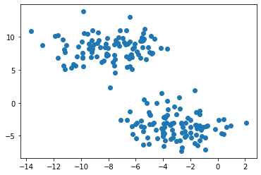
Clustering refers to the task of separating this data set into the two natural “blobs.” K-means is a very common way to achieve this task, which has good performance on circular-ish blobs like these:

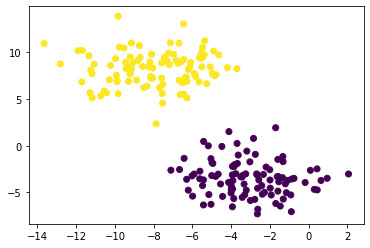
from sklearn.cluster import KMeans
km = KMeans(n_clusters = 2)
km.fit(X)

plt.scatter(X[:,0], X[:,1], c = km.predict(X))

Prefix II. Harder Clustering

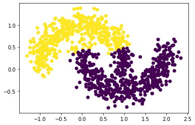
That was all well and good, but what if our data is “shaped weird”? Here, we can use the function make_moons supported by python to make the moonlike clusters:

np.random.seed(1234)
n = 200
X, y = datasets.make_moons(n_samples=n, shuffle=True, noise=0.05, random_state=None)
plt.scatter(X[:,0], X[:,1])

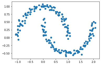
Similar as in Intro, can still make out two meaningful clusters in the data, but now they aren’t blobs but crescents. As before, the Euclidean coordinates of the data points are contained in the matrix X, while the labels of each point are contained in y. Now k-means won’t work so well, because k-means is, by design, looking for circular clusters.

km = KMeans(n_clusters = 2)
km.fit(X)
plt.scatter(X[:,0], X[:,1], c = km.predict(X))

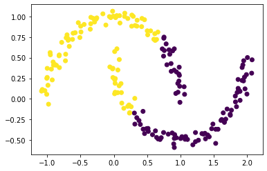
Clearly from the figure above, the clustering went wrong with the k-Means algorithm.

As will suggest below, spectral clustering is able to correctly cluster the two crescents. The following parts shows how to derive and implement spectral clustering.

Part A: Similarity Matrix Construction

In this part, construct an similarity matrix A, where n is the number of data points in the created cluster plot

First, clarify and define the similarity matrix needed here:

• The matrix construction should be based on another external parameter epsilon. Specifically, for each entry A[i,j] of A, the value should be equal to one if data point i is within the distance epsilon of data point j, which is to say,

• Moreover, the diagonal entries A[i,i] should all be equal to zero.

Now let’s start constructing the matrix:

For this part, I specified the value epsilon = 0.4. Also, to be more convenient for function construction, I used the function pairwise_distance from sklearn.metrics module, which could compute the euclidean distance between specified data points i and j.

epsilon = 0.4
from sklearn.metrics import pairwise_distances

To construct the similarity matrix A, I construct a function similarity_matrix_construction, which inputs the set of data points X and the epsilon value. Below is the function def.

def similarity_matrix_construction(X, epsilon):
  """
  Construct a similarity matrix indicator for whether each X[i]
  and X[j] are less than epsilon apart. Also, diagonal entries
  should all be zero for the desired output matrix.

  Input
  --------
  X: all data points informations
  epsilon: the maximum distance to be accepted

  Output
  --------
  A: the desired similarity matrix
  """
  # get dimension
  n = X.shape[0]
  # create empty matrix
  A = np.ndarray(shape = (n, n))
  # create matrix of distances using pairwise_distances
  # note: pairwise distances create a matrix D with D_ij as
  # distance between point X[i] and X[j]
  D = pairwise_distances(X, metric = 'euclidean')
  # now try to fill in A with information in D and epsilon
  A[D < epsilon**2] = 1
  A[D >= epsilon**2] = 0
  # empty the diagonal entries
  np.fill_diagonal(A, 0)
  # return similarity matrix
  return A

Now, store such similarity matrix as A for further use, and visualize the matrix:

A = similarity_matrix_construction(X, epsilon)
A

array([[0., 0., 0., ..., 0., 0., 0.],
       [0., 0., 0., ..., 0., 0., 0.],
       [0., 0., 0., ..., 0., 0., 0.],
       ...,
       [0., 0., 0., ..., 0., 0., 1.],
       [0., 0., 0., ..., 0., 0., 0.],
       [0., 0., 0., ..., 1., 0., 0.]])

The matrix A now contains information about which points are near (within distance epsilon) which other points.

Part B: Clustering Data Points - Binary Norm Cut Objective of Similarity Matrix

This part pose the task of clustering the data points in X as the task of partitioning the rows and columns of A.

B.0 Introduce the Concept of Binary Norm Cut Objective

To do spectral clustering, a key point is to find a small binary normcut objective. The binary norm cut objective of a matrix A with clusters clusters and is defined as:

In this expression,

• the cut term of clusters and is defined as the sum over all entries of , which needs to satisfy the conditions that i) the entries’ row indices i belongs to cluster , and ii) the column indices j belongs to cluster .
• The volume of a cluster is defined as the size of the cluster.

A pair of clusters and is considered to be a pair of “good” clstering when is small. The below parts would also partially show why having small binary norm cut objective is important by calculation based on real data.

B.1 The Cut Term

In this part, I’ll write a function called cut(A,y) to compute the cut term.

The cut term , by definition, calculates total number of datapoints pairs , such that i is in cluster and j is in , and that they are within epsilon distance apart. Having a small value for cut term would means, generally speaking, that clusters and are distance apart, which means that the clustering is somehow clear with less mismatches and mixings.

Now, write a python function cut(A, y) to directly calculate the cut term.

def cut(A, y):
  """
  calculate cut term with sim matrix A and
  the cluster-specifying vector y.

  Input
  --------
  A: the similarity matrix created
  y: the cluster-specifying vector, 0 or 1 valued entries
  
  Output
  --------
  cut: the cut term
  """
  # create the two clusters
  C0 = np.where(y == 0)[0]
  C1 = np.where(y == 1)[0]
  # calculate cut sum
  cut = 0
  for i in C0:
    for j in C1:
      cut += A[i, j]
  return cut

def cut(A, y):
  """
  calculate cut term with sim matrix A and
  the cluster-specifying vector y.

  Input
  --------
  A: the similarity matrix created
  y: the cluster-specifying vector, 0 or 1 valued entries
  
  Output
  --------
  cut: the cut term
  """
  # create the two clusters
  C0 = np.where(y == 0)[0]
  C1 = np.where(y == 1)[0]
  # calculate cut sum
  cut = 0
  for i in C0:
    for j in C1:
      cut += A[i, j]
  return cut

Below is an example calculation of the cut objectives. The true clusters refers y created in the cluster creation process, and the random clusters refers a vector named random, which has the same objective as y except that it is created totally at random. With such definition, we would expect the true cut to be lower than the random cut, as true clustering should work out better than the random clustering (which is supposed to be totally random and thus has bad clusters) selection among all datapoints.

# cut with true cluster y
true_cluster_cut = cut(A, y)
# cut with random cluster vector
np.random.seed(9999)
random = np.random.randint(2, size = A.shape[0])
random_cluster_cut = cut(A, random)
# find the two values with print
print("The cut objective for the true cluster is:", true_cluster_cut)
print("The cut objective for the random cluster is:", random_cluster_cut)

The cut objective for the true cluster is: 0.0
The cut objective for the random cluster is: 383.0

From the result above, as the true cut is 0, which is really nice and much more lower than the random clustering, it shows that this part of the cut objective indeed favors the true clusters over the random ones.

B.2 The Volume Term

In this part, I’ll write a function called vols(A,y) which computes the volumes of and ., returning them as a tuple. (for example, v0, v1 = vols(A,y))

As defined in part B.0, the volume of a cluster is simply the size of the cluster. With the definition of similarity matrix, the calculation could simply be done by summing entries over matrix A, which is direct. Below is the function def vols(A, y) of calculating the volumes of both cluster and .

def vols(A,y):
  """
  compute the volume of cluster C0 and C1 of
  the similarity matrix A specified by y

  Input
  --------
  A: the similarity matrix created
  y: the cluster-specifying vector, 0 or 1 valued entries
  
  Output
  --------
  (C0_vol, C1_vol): the volumes of clusters C0 and C1
  """
  # create a matrix d to store row sums of A
  d = A.sum(axis = 0)
  # find C0_vol and C1_vol by indexing sums
  C0_vol = d[y == 0].sum()
  C1_vol = d[y == 1].sum()
  # return output
  return (C0_vol, C1_vol)

def vols(A,y):
  """
  compute the volume of cluster C0 and C1 of
  the similarity matrix A specified by y

  Input
  --------
  A: the similarity matrix created
  y: the cluster-specifying vector, 0 or 1 valued entries
  
  Output
  --------
  (C0_vol, C1_vol): the volumes of clusters C0 and C1
  """
  # create the two clusters
  C0 = np.where(y == 0)[0]
  C1 = np.where(y == 1)[0]
  # calculate volume of C0 and C1
  C0_vol = np.sum([np.sum(A[i, ]) for i in C0])
  C1_vol = np.sum([np.sum(A[j, ]) for j in C1])
  # return volumes
  return (C0_vol, C1_vol)

B.3 The Norm Cut Calculation

In this part, I’ll write a function called normcut(A,y), which uses cut(A,y) and vols(A,y) to compute the binary normalized cut objective of a matrix A with clustering vector y.

Based on equationed definition mentioned in part B.0, can calculate the Norm Cut.

Below is the function def of normcut(A, y):

def normcut(A, y):
  """
  calculate the normcut of cluster C0 and C1 of
  the similarity matrix A specified by y

  Input
  --------
  A: the similarity matrix created
  y: the cluster-specifying vector, 0 or 1 valued entries
  
  Output
  --------
  normcut: the normcut of clusters C0 and C1
  """
  vol_c0, vol_c1 = vols(A, y)
  normcut = cut(A, y) * (1 / vol_c0 + 1 / vol_c1)
  return normcut

B.4 Norm Cut Comparison

Now, similar as part B.2, compare the calculated norm cut objective on both y and random to conclude that the norm cut objective also favors the true clusters over the random ones, as better clustering is supposed to have a lower normcut objective, similar as the cut objective.

• Why?: In this way, could see the normcut objective as a weighted version of the cut objective, and thus better normcut should have lower value to show that the two clusters are successfully separated, similarly with the understanding in part B.2).

# cut with true labels y
true_labels_normcut = normcut(A, y)
# cut with fake labels vector
fake_labels_normcut = normcut(A, random)
# find the two values with print
print("The normcut objective for the true cluster is:", true_labels_normcut)
print("The normcut objective for the random cluster is:", fake_labels_normcut)

The normcut objective for the true cluster is: 0.0
The normcut objective for the random cluster is: 1.0074122463651651

From the result, the normcut objective for true cluster is 0, which is way lower than about 1 of the one for random cluster. Therefore, can conclude that the norm cut objective also favors the true clusters over the random ones.

Part C: Find Small Normcut - The (D, z) Definition of Normcut

This part helps to prove that the value y for making normcut(A, y) small can be calculated using a specified equation that could be calculated directly as follows:

C.1 Concepts and Process Specification

For success clustering, need to find y such that normcut(A,y) is small. However, from the definition in part B, it is hard to do minimization and find a small normcut term. This part actually shows that instead of the definition in part B, we can use another definition, as shown as the equation def above, which is a purely linear algebra well-defined equation, such that is direct for the minimization problem.

Below is a set of mathematical definitions of the above term:

1. is defined as:

2. the matrix D is:

the diagonal matrix with nonzero entries , and where is the degree (row-sum) from before.

3. Show that the defined equation holds:

C.1 Proof with Programming

Now, let’s do the computation process, in the following part, I’ll:

1. Write a function called transform(A,y): compute the appropriate vector given A and y, using the formula above.

def transform(A,y):
  """
  calculate z-vector of cluster C0 and C1 of
  the similarity matrix A specified by y

  Input
  --------
  A: the similarity matrix created
  y: the cluster-specifying vector, 0 or 1 valued entries
  
  Output
  --------
  z: the z-vector of clusters C0 and C1
  """
  z = np.zeros(y.shape[0])
  vol_c0, vol_c1 = vols(A, y)
  z[y == 0] = 1 / vol_c0
  z[y == 1] = -1 / vol_c1
  return z

2. Construct the matrix D from A

def D_construction(A):
  """
  calculate the desired diagonal rowsum-valued matrix D from A
  """
  # create vector storing all rowsums of sim matrix A
  A_row_sum = [np.sum(A[i, ]) for i in np.arange(A.shape[0])]
  # construct and return result D
  D = np.diag(A_row_sum)
  return D

3. Show that the equation (want to prove) holds

Here the equation above is exact, but computer arithmetic is not! The python function np.isclose(a,b) is a good way to check if a is “close” to b, in the sense that they differ by less than the smallest amount that the computer is (by default) able to quantify.

Below is the total construction process use functions in 1 and 2 as well as checking whether the equation holds (LHS = RHS):

# calculate the diagonal rowsum-valued matrix D
D = D_construction(A)
# calculate z-vector
z = transform(A, y)
# find the right hand side of the equation
normcut_with_D_z = 2 * z@(D-A)@z / (z@D@z)
# check validility and correctness of the equation
# note: normcut(A, y) calculate left hand side of the eqn
np.isclose(normcut(A, y), normcut_with_D_z)

True

Therefore, successfully proved that the equation holds.

Part D: Minimize Normcut Objective

Note: the idea of this part is sourced from Phil’s Blog Post 2 instruction.

As shown in last part, the normcut function

Therefore, find small normcut objective now becomes the mathematical optimization problem of minimizing the function:

subject to the condition . It’s actually possible to bake this condition into the optimization, by substituting for the orthogonal complement of relative to . Below function orth_obj function handles this porblem.

def orth(u, v):
    return (u @ v) / (v @ v) * v

e = np.ones(n) 

d = D @ e

def orth_obj(z):
    z_o = z - orth(z, d)
    return (z_o @ (D - A) @ z_o)/(z_o @ D @ z_o)

Now, use the function minimize from scipy.optimize module to minimize the function orth_obj with respect to .

from scipy.optimize import minimize

minimized_contents = minimize(orth_obj, z)
minimized_contents.keys()

dict_keys([‘fun’, ‘jac’, ‘hess_inv’, ‘nfev’, ‘njev’, ‘status’, ‘success’, ‘message’, ‘x’, ‘nit’])

Now, can see that the minimized contents contains a lot of components, the desired data result we want is actually from the content 'x'. Therefore, store the minimized z as z_min with the 'x' key from minimized_contents:

z_min = minimized_contents.x

Part E: Scattering Spectral Clusters with Minimized Normcut

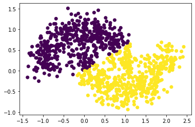
From part d, get that z_min is the clustering that minimize the Normcut. Now, plot the scatter plot by changing coloring to z_min:

plt.scatter(X[:,0], X[:,1], c = z_min)

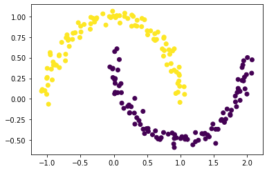
Nice! With the spectral clustering, now the scatters are with the correct clusters based on z_min.

Part F: Implicit Optimization of Orthogonal Objectives

From part d, we actually do the explicit optimization using the function minimize supported by python. However, it is way too complicated sometimes when programming. Actually, the minimization problem can be solved using eigenvalues and eigenvectors of matrices.

F.0 Concept Introduction of Clarification

Note: this part is sourced from Phil’s Blog Post 2 Instruction as a proof and explanation on how the eigenvector method potentially works.

Recall that what we would like to do is minimize the function

with respect to , subject to the condition .

The Rayleigh-Ritz Theorem states that the minimizing must be the solution with smallest eigenvalue of the generalized eigenvalue problem

which is equivalent to the standard eigenvalue problem

where is actually the eigenvector with smallest eigenvalue of the matrix .

Therefore, the vector that we want must be the eigenvector with the second-smallest eigenvalue.

F.1 Eigenvector Method Implementation by Python Programming

Based on the above explanation, now we can construct the optimization process in python:

1. Construct the matrix , which is often called the (normalized) Laplacian matrix of the similarity matrix .

To construct the Laplacian matrix, I wrote a function names L_construction, which input a matrix A and output its Laplacian matrix. Below is the function def:

def L_construction(A):
  """
  Construct a similarity matrix indicator for whether each X[i]
  and X[j] are less than epsilon apart. Also, diagonal entries
  should all be zero for the desired output matrix.

  Input
  --------
  X: all data points informations
  epsilon: the maximum distance to be accepted

  Output
  --------
  A: the desired similarity matrix
  """
  # create vector storing all rowsums of sim matrix A
  A_row_sum = [np.sum(A[i, ]) for i in np.arange(A.shape[0])]
  # create the diagonal rowsum-valued matrix D
  D = np.diag(A_row_sum)
  # calculate L
  L = np.linalg.inv(D)@(D - A)
  return L

2. Find the eigenvector corresponding to its second-smallest eigenvalue, and call it z_eig.

First, I wrote a function for finding the second smallest eigenvalue and its corresponding eigenvector. The function second_smallest_eigen inputs the desired Laplacian matrix, and outputs the second smallest eigenvalue and its corresponding eigenvector as a tuple. Below is the function construction:

def second_smallest_eigen(L):
  """
  return second smallest eigenvalue and corresponding eigenvector
  """
  # Lam gives the eigenvalues of L, U gives the eigenvectors (as columns)
  Lam, U = np.linalg.eig(L)

  # eigenvector with second-smallest eigenvalue
  # spoiler, you're going to need this one soon!
  ix = Lam.argsort()
  Lam, U = Lam[ix], U[:,ix]

  # 2nd smallest eigenvalue and corresponding eigenvector
  return (Lam[1], U[:,1])

Now, with the above function as well as the L_construction function in 1, can calculate the optimized z based on this second smallest eigenvector, name it as z_eig. Below is the construction process of z_eig.

# calculate L
L = L_construction(A)
# calculate 2nd smallest eigenvalue and corresponding eigenvector
Lam[1], U[:,1] = second_smallest_eigen(L)
# store the 2nd smallest-eigenvalued eigenvector as z_eig
z_eig = U[:,1]

3. Plot the data again, using the sign of z_eig as the color.

Now, with z_eig, can do the plotting process similar as part e:

plt.scatter(X[:,0], X[:,1], c = z_eig)

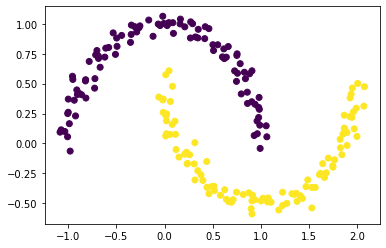
And again, the scattering is correct!

Part G: Spectral Clustering

This part writes a function spectral_clustering(X, epsilon), which basically do the whole spectral clustering process, which is a previous process based summary.

The function spectral_clustering(X, epsilon) inputs the data points information X and the given distance threshold epsilon, and outputs the spectral clustering labeling vector labels.

Below is the definition of this function:

def spectral_clustering(X, epsilon):
  """
  Performs spectral clustering based on input data X 
  and the distance threshold epsilon, returning 
  an array of binary labels indicating whether
  data point i is in group 0 or group 1.

  The process is concatenated as four steps:
  1. Construct the similarity matrix.
  2. Construct the Laplacian matrix.
  3. Compute the eigenvector with second-smallest eigenvalue of the Laplacian matrix.
  4. Return labels based on this eigenvector.

  Input
  --------
  X: all data points informations
  epsilon: the maximum distance to be accepted

  Output
  --------
  labels: array of binary labels indicating whether data point i is in group 0 or 1
  """

  # Step 1: Construct the similarity matrix.
  A = similarity_matrix_construction(X, epsilon)
  # Step 2: Construct the Laplacian matrix.
  L = L_construction(A)
  # Step 3: Compute the eigenvector with second-smallest eigenvalue of L
  sec_small_eigvalue, sec_small_eigvec = second_smallest_eigen(L)
  # Step 4: Return labels based on this eigenvector.
  labels = sec_small_eigvec
  labels[sec_small_eigvec >= 0] = 1
  labels[sec_small_eigvec < 0] = 0
  return labels

Now, try to visualize the result labels to make sure the function works, recall that epsilon = 0.4 is already defined:

spectral_clustering(X, epsilon)

array([1., 1., 0., 0., 0., 0., 0., 0., 1., 1., 1., 0., 1., 1., 1., 1., 1.,
       0., 0., 0., 1., 1., 1., 0., 0., 1., 0., 1., 1., 0., 0., 1., 1., 1.,
       1., 1., 0., 1., 1., 0., 1., 0., 0., 0., 0., 0., 0., 1., 1., 1., 0.,
       0., 1., 1., 0., 0., 1., 1., 1., 0., 0., 0., 1., 0., 1., 0., 0., 0.,
       0., 1., 1., 1., 1., 0., 0., 0., 1., 0., 1., 0., 0., 0., 0., 1., 1.,
       1., 1., 0., 0., 0., 0., 1., 0., 0., 1., 1., 1., 1., 0., 0., 1., 1.,
       1., 0., 1., 1., 0., 0., 1., 1., 0., 0., 0., 1., 0., 0., 0., 0., 1.,
       1., 1., 0., 1., 1., 1., 0., 1., 0., 1., 1., 0., 0., 0., 0., 1., 1.,
       1., 1., 1., 1., 1., 1., 0., 0., 1., 0., 0., 0., 0., 0., 0., 0., 0.,
       1., 1., 0., 1., 0., 0., 0., 1., 1., 0., 0., 1., 1., 1., 0., 0., 0.,
       1., 0., 1., 1., 1., 0., 0., 0., 0., 1., 1., 0., 0., 1., 1., 1., 0.,
       1., 1., 1., 0., 1., 0., 1., 1., 1., 1., 0., 0., 0.])

Seems that the function works properly! Now we can work on the graph visualizations to see whether clustering are correctly defined.

Part H: Mooned Clustering with Different Noise

This part plots some mooned clustering plots based on different noise levels. To specify, this part fixes number of samples to 1000, and fix epsilon to 0.5

With the spectral_clustering function defined, can plot mooned clusters based on spectral clustering with different noise.

First, write a function to do the whole plotting process, with different inputted noise. Below is the function def:

np.random.seed(9999) # set random seed
def plot_scatter_with_noise(noise):
  """
  plot based on different input noises
  """
  X, y = datasets.make_moons(n_samples=1000, shuffle=True, noise=noise, random_state=None)
  labels = spectral_clustering(X, epsilon = 0.5)
  plt.scatter(X[:,0], X[:,1], c = labels)

Now, plot with different noises:

1. Noise Level = 0.05

plot_scatter_with_noise(0.05)

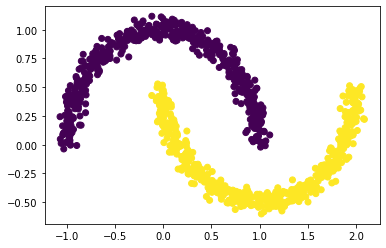
2. Noise Level = 0.10

plot_scatter_with_noise(0.1)

3. Noise Level = 0.15

plot_scatter_with_noise(0.15)

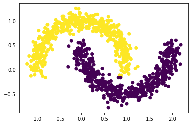
4. Noise Level = 0.20

plot_scatter_with_noise(0.2)

As can see from the above plots, as the noise increases, the “diameter” of the moon increases, and the two moons are more likely to mix between each other. In other words, as noise increases, the general distances between two clusters are decreasing, making the clustering process harder (need lower epsilons).

Part I: More Confirmation in Correctness - Clustering the Bull’s Eye

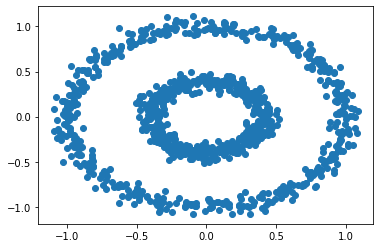
Now let’s see that the clustering process works on the bull’s eye.

The bull’s eye clusters is created and visualized as follows:

n = 1000
X, y = datasets.make_circles(n_samples=n, shuffle=True, noise=0.05, random_state=None, factor = 0.4)
plt.scatter(X[:,0], X[:,1])

With comparison, first do the clusterning based on the K-Means method:

km = KMeans(n_clusters = 2)
km.fit(X)
plt.scatter(X[:,0], X[:,1], c = km.predict(X))

Clearly can see, the k-means methods does not correctly clustering the bull’s eye.

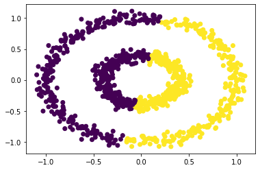
Now let’s try with spectral clustering method, with epsilon = 0.6:

plt.scatter(X[:,0], X[:,1], c = spectral_clustering(X, epsilon = 0.6))

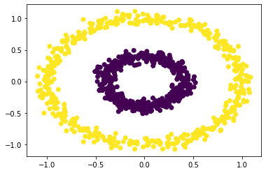
Yes! Our spectral clustering algorithm correctly clusters the bull’s eyes with specified epsilon value of 0.6, which is a correct but might not unique solution to make the correct bull’s eye spectral clustering.