
Assignment - Blog Post 1
This blog post includes some graphics related to global climate change. Data sourced from the NOAA climate data.
§1. Database Creation
1.1: Data Importing
For the temperature dataset, first do the visualization. The real importing part happens together with the database creation.
import pandas as pd
temperatures = pd.read_csv("/Users/xuyan/Desktop/temps.csv")
temperatures.head()
| ID | Year | VALUE1 | VALUE2 | VALUE3 | VALUE4 | VALUE5 | VALUE6 | VALUE7 | VALUE8 | VALUE9 | VALUE10 | VALUE11 | VALUE12 | |
|---|---|---|---|---|---|---|---|---|---|---|---|---|---|---|
| 0 | ACW00011604 | 1961 | -89.0 | 236.0 | 472.0 | 773.0 | 1128.0 | 1599.0 | 1570.0 | 1481.0 | 1413.0 | 1174.0 | 510.0 | -39.0 |
| 1 | ACW00011604 | 1962 | 113.0 | 85.0 | -154.0 | 635.0 | 908.0 | 1381.0 | 1510.0 | 1393.0 | 1163.0 | 994.0 | 323.0 | -126.0 |
| 2 | ACW00011604 | 1963 | -713.0 | -553.0 | -99.0 | 541.0 | 1224.0 | 1627.0 | 1620.0 | 1596.0 | 1332.0 | 940.0 | 566.0 | -108.0 |
| 3 | ACW00011604 | 1964 | 62.0 | -85.0 | 55.0 | 738.0 | 1219.0 | 1442.0 | 1506.0 | 1557.0 | 1221.0 | 788.0 | 546.0 | 112.0 |
| 4 | ACW00011604 | 1965 | 44.0 | -105.0 | 38.0 | 590.0 | 987.0 | 1500.0 | 1487.0 | 1477.0 | 1377.0 | 974.0 | 31.0 | -178.0 |
Now, import and visualize the countries dataset:
# this is the countries data
countries_url = "https://raw.githubusercontent.com/mysociety/gaze/master/data/fips-10-4-to-iso-country-codes.csv"
countries = pd.read_csv(countries_url)
countries.head()
| FIPS 10-4 | ISO 3166 | Name | |
|---|---|---|---|
| 0 | AF | AF | Afghanistan |
| 1 | AX | - | Akrotiri |
| 2 | AL | AL | Albania |
| 3 | AG | DZ | Algeria |
| 4 | AQ | AS | American Samoa |
Now, import and visualize the stations dataset:
# this is the stations data
stations_url = "https://raw.githubusercontent.com/PhilChodrow/PIC16B/master/datasets/noaa-ghcn/station-metadata.csv"
stations = pd.read_csv(stations_url)
stations.head()
| ID | LATITUDE | LONGITUDE | STNELEV | NAME | |
|---|---|---|---|---|---|
| 0 | ACW00011604 | 57.7667 | 11.8667 | 18.0 | SAVE |
| 1 | AE000041196 | 25.3330 | 55.5170 | 34.0 | SHARJAH_INTER_AIRP |
| 2 | AEM00041184 | 25.6170 | 55.9330 | 31.0 | RAS_AL_KHAIMAH_INTE |
| 3 | AEM00041194 | 25.2550 | 55.3640 | 10.4 | DUBAI_INTL |
| 4 | AEM00041194 | 24.4300 | 54.4700 | 3.0 | ABU_DHABI_BATEEN_AIR |
1.2: Database Settling
First, create the database:
import sqlite3
conn = sqlite3.connect("temps.db")
# store the path for temperature csv file
temps = "/Users/xuyan/Desktop/temps.csv"
df_iter = pd.read_csv(temps, chunksize = 100000)
df = df_iter.__next__()
Now, reshape the dataset to store as the temperature dataset
# reshape function:
def prepare_df(df):
    df = df.set_index(keys=["ID", "Year"])
    df = df.stack()
    df = df.reset_index()
    df = df.rename(columns = {"level_2"  : "Month" , 0 : "Temp"})
    df["Month"] = df["Month"].str[5:].astype(int)
    df["Temp"]  = df["Temp"] / 100
    return(df)

# reshaping process:
df = prepare_df(df)
df.head()
| ID | Year | Month | Temp | |
|---|---|---|---|---|
| 0 | ACW00011604 | 1961 | 1 | -0.89 |
| 1 | ACW00011604 | 1961 | 2 | 2.36 |
| 2 | ACW00011604 | 1961 | 3 | 4.72 |
| 3 | ACW00011604 | 1961 | 4 | 7.73 |
| 4 | ACW00011604 | 1961 | 5 | 11.28 |
Now, write the three datasets to the database:
# 1. write temperature dataset to database
df_iter = pd.read_csv(temps, chunksize = 100000)
for df in df_iter:
    df = prepare_df(df)
    df.to_sql("temperatures", conn, if_exists = "append", index = False)

# 2. write stations dataset to database
stations.to_sql("stations", conn, if_exists = "replace", index = False)

# 3. write countries dataset to database
countries.to_sql("countries", conn, if_exists = "replace", index = False)
1.3: Database Precheck
Now, visualize the general information of the dataset:
- Datasets in Database
cursor = conn.cursor()
cursor.execute("SELECT name FROM sqlite_master WHERE type='table'")
print(cursor.fetchall())
[('temperatures',), ('stations',), ('countries',)]
- Datasets Contents in Database
cursor.execute("SELECT sql FROM sqlite_master WHERE type='table';")

for result in cursor.fetchall():
    print(result[0])
CREATE TABLE "temperatures" (
"ID" TEXT,
  "Year" INTEGER,
  "Month" INTEGER,
  "Temp" REAL
)
CREATE TABLE "stations" (
"ID" TEXT,
  "LATITUDE" REAL,
  "LONGITUDE" REAL,
  "STNELEV" REAL,
  "NAME" TEXT
)
CREATE TABLE "countries" (
"FIPS 10-4" TEXT,
  "ISO 3166" TEXT,
  "Name" TEXT
)
§2. Query Function
This Query function
query_climate_database()inputs specified country name, start year and end year for consideration, specified month to look on, and return a dataset to write on.
- Function Input - Dataset Restriction Contents:
country, a string giving the name of a country for which data should be returned.year_beginandyear_end, two integers giving the earliest and latest years for which should be returned.month, an integer giving the month of the year for which should be returned.
- Output Dataset Contents:
- The station name.
- The latitude of the station.
- The longitude of the station.
- The name of the country in which the station is located.
- The year in which the reading was taken.
- The month in which the reading was taken.
- The average temperature at the specified station during the specified year and month.
2.1: Function Construction:
Now, start writing the function:
def query_climate_database(country, year_begin, year_end, month):

    """
    function returning a dataset of temperature readings for
    the specified country, in the specified date range, in
    the specified month of the year.

    Input
    --------
    country: string, tell which country for database to return
    year_begin: int, earliest year to be returned
    year_end: int, last year to be returned
    month: int, month of the year to be returned

    Output
    --------
    out: dataframe of temperature readings for the specified
        country, in the specified date range, in the specified
        month of the year.
    """

    # Write SQL command to satisfy with the output type
    # SELECT: necessay column names
    # From & LEFT JOIN * 2: "merge" the three datasets in form of temperature dataset
    # WHERE: specified output places
    cmd = \
    f"""
    SELECT S.name, S.latitude, S.longitude, C.Name, T.year, T.month, T.temp
    FROM temperatures T
    LEFT JOIN stations S ON T.id = S.id
    LEFT JOIN countries C ON SUBSTRING(T.id, 1, 2) = C.`FIPS 10-4`
    WHERE C.name="{country}" AND T.month={month} AND T.year>={year_begin} AND T.year<={year_end}
    """

    # Write dataset from SQL Query
    out = pd.read_sql_query(cmd, conn)

    return out
- A NOTE from self-learning of SQL: For the second left join command, can be done via either
=orLIKE. However,LIKEseemed to be slower compared to the direct comparison with theSUBSTRINGcommand via=.
2.2: Function Check
Check that the function output aligns with the example output:
query_climate_database(country = "India",
                       year_begin = 1980,
                       year_end = 2020,
                       month = 1)
| NAME | LATITUDE | LONGITUDE | Country | Year | Month | Temp | |
|---|---|---|---|---|---|---|---|
| 0 | PBO_ANANTAPUR | 14.583 | 77.633 | India | 1980 | 1 | 23.48 |
| 1 | PBO_ANANTAPUR | 14.583 | 77.633 | India | 1981 | 1 | 24.57 |
| 2 | PBO_ANANTAPUR | 14.583 | 77.633 | India | 1982 | 1 | 24.19 |
| 3 | PBO_ANANTAPUR | 14.583 | 77.633 | India | 1983 | 1 | 23.51 |
| 4 | PBO_ANANTAPUR | 14.583 | 77.633 | India | 1984 | 1 | 24.81 |
| ... | ... | ... | ... | ... | ... | ... | ... |
| 3147 | DARJEELING | 27.050 | 88.270 | India | 1983 | 1 | 5.10 |
| 3148 | DARJEELING | 27.050 | 88.270 | India | 1986 | 1 | 6.90 |
| 3149 | DARJEELING | 27.050 | 88.270 | India | 1994 | 1 | 8.10 |
| 3150 | DARJEELING | 27.050 | 88.270 | India | 1995 | 1 | 5.60 |
| 3151 | DARJEELING | 27.050 | 88.270 | India | 1997 | 1 | 5.70 |
3152 rows × 7 columns
Nice! Now get the exact database as desired.
- Small remark: when want to rewrite the whole database, simply delete it from the files.
§3. Geographical Scatter Function
This function
temperature_coefficient_plot()accept five explicit arguments, and an undetermined number of keyword arguments; and output an interactive geographic scatterplot, with a point for each station, such that the color of the point reflects an estimate of the yearly change in temperature during the specified month and time period at that station.
- Function Input - Dataset Restriction Contents:
country, a string giving the name of a country for which data should be returned.year_beginandyear_end, two integers giving the earliest and latest years for which should be returned.month, an integer giving the month of the year for which should be returned.min_obs, the minimum required number of years of data for any given station. Only data for stations with at leastmin_obsyears worth of data in the specified month should be plotted; the others should be filtered out.df.transform()plus filtering is a good way to achieve this task.**kwargs, additional keyword arguments passed topx.scatter_mapbox(). These can be used to control the colormap used, the mapbox style, etc.
- Output Contents:
- an interactive geographic scatterplot constructed using Plotly Express as described in
INTROpart.
- an interactive geographic scatterplot constructed using Plotly Express as described in
3.1: Function Construction
First, import necessary packages:
from sklearn.linear_model import LinearRegression
from plotly import express as px
from matplotlib import pyplot as plt
As illustrated in the lecture, there’s a coefficient funciton for use in the plotting function:
def coef(data_group):
    x = data_group[["Year"]] # 2 brackets because X should be a df
    y = data_group["Temp"]   # 1 bracket because y should be a series
    LR = LinearRegression()
    LR.fit(x, y)
    return LR.coef_[0]
Now, start writing the plotting-return function:
def temperature_coefficient_plot(country, year_begin, year_end, month, min_obs, **kwargs):

    """
    plot heat-colored map of stations in a specific country
    and specified month, with specified time interval

    Input
    --------
    country: string, tell which country for database to return
    year_begin: int, earliest year to be returned
    year_end: int, last year to be returned
    month: int, month of the year to be returned
    min_obs: the minimum years of observations
    **kwargs: random keyword arguments to be applied in the plotting

    Output
    --------
    The temperature plot
    """

    # 1. write desired dataset from database with query function
    df = query_climate_database(country, year_begin, year_end, month)

    # 2. only keep stations with years more than min_obs
    # store the number of years considered as year_num variable for each row entry
    num_years = df.groupby(["NAME"])["Year"].transform("count")
    # cut the dataset with those stations only greater than min_obs
    df = df[num_years >= min_obs]

    # 3. get yearly temperature average increase dataset
    yearly_temp_increase = df.groupby(["NAME", "Month"]).apply(coef).reset_index()
    # rename column as yearly_temperature_increase
    yearly_temp_increase = yearly_temp_increase.rename(columns={0: "Estimated Yearly Increase (°C)"})

    # 4. append geographic spotpoints (LATI & LONG)
    # create temporary dataset with only geographic INFO
    spots = df[["NAME", "LATITUDE", "LONGITUDE"]].drop_duplicates()
    # reset indexing
    spots = spots.reset_index().drop(["index"], axis = 1)
    # append spotpoints locations by merging two datasets
    final = pd.merge(yearly_temp_increase, spots, on = ["NAME"])

    # 5. create the graph
    fig = px.scatter_mapbox(final, hover_name = "NAME", lat = "LATITUDE", lon = "LONGITUDE",
                            color = "Estimated Yearly Increase (°C)",
                            **kwargs)
    return fig
3.2: Sample Output Check
For example, create a plot of estimated yearly increases in temperature during the month of January, in the interval 1980-2020, in India.
color_map = px.colors.diverging.RdGy_r # choose a colormap
fig = temperature_coefficient_plot("India", 1980, 2020, 1,
                                   min_obs = 10,
                                   zoom = 2,
                                   mapbox_style="carto-positron",
                                   color_continuous_scale=color_map)
fig.show()
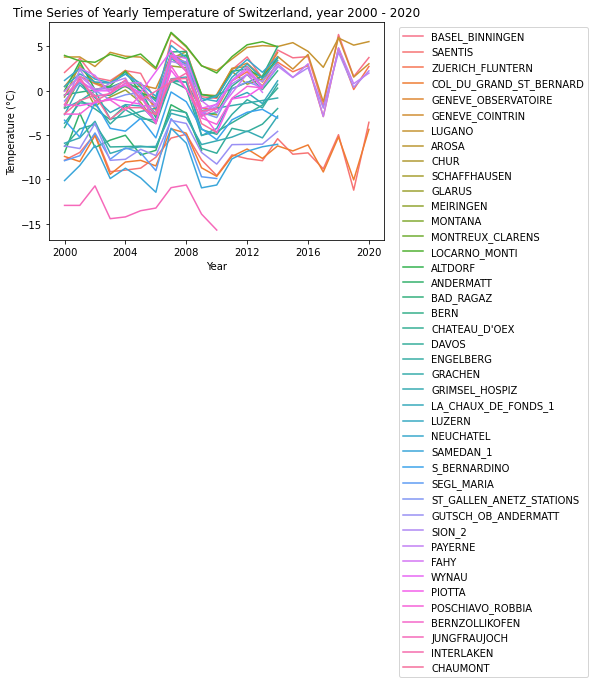
§4. Time Series Temperature Plot of Switzerland from 2000 to 2020
4.1 Time Series Plotting Function
The function
yearly_time_series_temperature()accept three explicit arguments; and output a time series plot, with a line representing one station, such that it plots all time series of temperatures of a country’s stations over a time interval on the same plot.
- Function Input:
country, a string giving the name of a country for which data should be returned.year_beginandyear_end, two integers giving the earliest and latest years for which should be returned.
- Output Contents:
- temperature time series of all stations of a given country within a specified time interval
Now, start to construct the function:
import seaborn as sns

def yearly_time_series_temperature(country, year_begin, year_end):
    """
    plot yearly time series plot of stations in a specific country
    with specified month, within a specified time interval (year)
    **mark: suppose the yearly temperature counted as January

    Input
    --------
    country: string, tell which country for database to return
    year_begin: int, earliest year to be returned
    year_end: int, last year to be returned

    Output
    --------
    The yearly time series plot
    """

    # write desired dataset from database with query function
    df = query_climate_database(country, year_begin, year_end, 1)
    # datetime transform (lecture note)
    df["Date"] = df["Year"].astype(str) + "-" + df["Month"].astype(str)
    df["Date"] = pd.to_datetime(df["Date"])

    # set title name:
    title_str = "Time Series of Yearly Temperature of " + country + ", year " + str(year_begin) + " - " + str(year_end)

    # create and set figures
    fig = sns.lineplot(data = df, x = "Date", y = "Temp", hue = "NAME")
    # switch legend place
    fig.legend(bbox_to_anchor= (1.03, 1))
    # set title, names of axis
    fig.set(xlabel = 'Year', ylabel = 'Temperature (°C)',
           title = title_str)

    return fig
4.2 Temperature Time Series of Switzerland Stations from 2000 to 2020
Now, use the function defined in 4.1, plot the time series to visualize the temperature changes of all switzerland stations in the time interval of 2000 - 2020.
yearly_time_series_temperature("Switzerland", 2000, 2020)
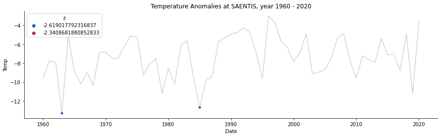
§5. Visualize Anomalies for a Given Station
5.1 Library Import and Z-score Function
An important feature for looking at anomalies is the z-score. Therefore, before writing the plotting function, the z-score function needs to be pre-defined.
Import necessary packages and define z-score function here:
from matplotlib import pyplot as plt
import numpy as np

# z-score function def
def z_score(x):
    m = np.mean(x)
    s = np.std(x)
    return (x - m)/s
5.2 Plotting Function Construction
The function
station_anomalies_plot()accept four explicit arguments; and output a time series plot with only one time series representing the specified station, together with anomalies given in the specified time series.
- Function Input:
country, a string giving the name of a country for which data should be returned.year_beginandyear_end, two integers giving the earliest and latest years for which should be returned.station, a string giving the name of the station for which to plot on
- Output Contents:
- a temperature time series plot of
Now, start to construct the function:
def station_anomalies_plot(country, year_begin, year_end, station):

    """
    plot station temperature time series together with anomalies
    within the given period, need to know country of the station

    Input
    --------
    country: string, tell which country for database to return
    year_begin: int, earliest year to be returned
    year_end: int, last year to be returned
    station: string, tell which station to look at

    Output
    --------
    The temperature time series of a given station with anomalies
    """

    # write desired dataset from database with query function
    df = query_climate_database(country, year_begin, year_end, 1)
    # datetime transform (lecture note)
    df["Date"] = df["Year"].astype(str) + "-" + df["Month"].astype(str)
    df["Date"] = pd.to_datetime(df["Date"])

    # calculate z-score and find anomalies
    df["z"] = df.groupby(["NAME", "Month"])["Temp"].transform(z_score)
    anomalies = df[np.abs(df["z"]) > 2]

    #plotting
    # create plot
    fig = plt.subplots(figsize = (15, 4))
    # time series line plot
    sns.lineplot(data = df[df["NAME"] == station],
                 x = "Date",
                 y = "Temp",
                 color = "lightgrey")
    # dot plotting anomalies
    sns.scatterplot(data = anomalies[anomalies["NAME"] == station],
                    x = "Date",
                    y = "Temp",
                    zorder = 100, # show the dots on top
                    hue = "z",
                    s = 30,
                    palette = "vlag")
    # set title
    plt.gca().set(title = f"Temperature Anomalies at {station}, year {year_begin} - {year_end}")
    sns.despine()
5.3 Data Visualization of Anomalies of the SAENTIS Station in Switzerland
Now, with the function construction in 5.2, plot the temperature time series of the SAENTIS station in Switzerland from 1960 to 2020 together with all anomalies within the time interval
station_anomalies_plot("Switzerland", 1960, 2020, "SAENTIS")
§6. Close Database
Last, close the database.
conn.close()
This is the end of this blog post! :)
I learned something really cool from my peer feedback!
I gave one of my peers a cool suggestion!